Exponential Equation Formulas – Exponent & Base Rules

Exponential Equation

An exponential equation is an equation in which variables appear as exponents. The general form is:

\[ a^{x} = b \]

Basic form:

\[ a^{x} = b, \quad a > 0, a \neq 1 \]

Solution:

\[ x = \log_{a} b \]

Properties of Exponents:

\(a^{m} \times a^{n} = a^{m+n}\)
\(\frac{a^{m}}{a^{n}} = a^{m-n}\)
\(\left(a^{m}\right)^{n} = a^{mn}\)
\(a^{0} = 1\)
\(a^{-n} = \frac{1}{a^{n}}\)

Natural Exponential Function:

\[ e^{x} = \lim_{n \to \infty} \left(1 + \frac{x}{n}\right)^n \]

Terminology

Base \(a\): The constant raised to a variable exponent.
Exponent \(x\): The variable or constant that serves as the power.
Logarithm: The inverse operation of exponentiation.
Natural base \(e\): An important mathematical constant approximately equal to 2.71828.

Applications

Modeling population growth and radioactive decay.
Compound interest calculations in finance.
Describing natural processes such as cooling and charging of capacitors.
Used in differential equations and complex analysis.

🔑

Key Formula - General Form

\[ a^x = b \]

\[ \text{where } a > 0, a \neq 1, \text{ and } b > 0 \]

🎯 What does this mean?

An exponential equation is one where the unknown variable appears as an exponent. These equations model rapid growth or decay phenomena and are fundamental in describing natural processes, financial calculations, and scientific relationships where rates of change are proportional to current values.

🧮

Solution Methods

Primary techniques for solving exponential equations:

\[ \text{Method 1: Same Base - } a^x = a^y \Rightarrow x = y \]

\[ \text{Method 2: Logarithms - } a^x = b \Rightarrow x = \log_a(b) \]

\[ \text{Method 3: Natural Log - } e^x = k \Rightarrow x = \ln(k) \]

\[ \text{Method 4: Change of Base - } x = \frac{\ln(b)}{\ln(a)} \]

📊

Common Types and Solutions

Standard exponential equation patterns:

\[ 2^x = 8 \Rightarrow 2^x = 2^3 \Rightarrow x = 3 \]

\[ 5^x = 125 \Rightarrow 5^x = 5^3 \Rightarrow x = 3 \]

\[ 3^x = 7 \Rightarrow x = \log_3(7) = \frac{\ln(7)}{\ln(3)} \]

\[ e^x = 20 \Rightarrow x = \ln(20) \]

🔄

Advanced Forms and Techniques

Complex exponential equations and methods:

\[ a^{f(x)} = a^{g(x)} \Rightarrow f(x) = g(x) \]

\[ a^x + b^x = c \text{ (requires substitution or graphing)} \]

\[ (a^x)^2 - k \cdot a^x + m = 0 \text{ (quadratic in } a^x \text{)} \]

\[ \text{Let } y = a^x, \text{ then solve quadratic in } y \]

📈

Growth and Decay Models

Real-world exponential equation applications:

\[ A(t) = A_0 \cdot e^{rt} \text{ (continuous growth/decay)} \]

\[ A(t) = A_0 \cdot (1 + r)^t \text{ (compound interest)} \]

\[ N(t) = N_0 \cdot e^{-\lambda t} \text{ (radioactive decay)} \]

\[ P(t) = \frac{L}{1 + ae^{-kt}} \text{ (logistic growth)} \]

🎯

Properties and Rules

Essential properties for solving exponential equations:

\[ a^m \cdot a^n = a^{m+n} \]

\[ \frac{a^m}{a^n} = a^{m-n} \]

\[ (a^m)^n = a^{mn} \]

\[ a^{-n} = \frac{1}{a^n} \]

🎯 Problem-Solving Strategy

When solving exponential equations, first identify if both sides can be expressed with the same base. If so, equate the exponents. If not, use logarithms to bring the variable down from the exponent. For complex forms, consider substitution to transform the equation into a familiar algebraic form.

\[ a^x = b \]

Standard exponential equation form with variable x in the exponent

\[ a \]

Base of the exponential - must be positive and not equal to 1

\[ x \]

Unknown variable appearing in the exponent position

\[ b \]

Result value - must be positive for real solutions

\[ \log_a(b) \]

Logarithm base a of b - the solution to a^x = b

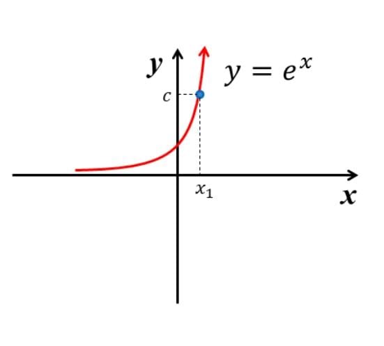
\[ e \]

Natural exponential base ≈ 2.718, commonly used in growth models

\[ \ln(x) \]

Natural logarithm - logarithm base e, inverse of e^x

\[ A_0 \]

Initial value in growth/decay models at time t = 0

\[ r \]

Growth rate (positive) or decay rate (negative) in exponential models

\[ t \]

Time variable in growth and decay applications

\[ \text{Substitution} \]

Technique using y = a^x to convert to algebraic equations

\[ \text{Same Base} \]

Method where both sides are expressed as powers of same base

🎯 Essential Insight: Exponential equations are like "power puzzles" - the key is getting the variable out of the exponent using logarithms or finding a common base! 🧮

🚀 Real-World Applications

💰 Finance & Economics

Compound Interest & Investment Growth

Banks use exponential equations to calculate compound interest, determine loan payoff times, and model investment growth over time periods

🧬 Biology & Medicine

Population Growth & Drug Decay

Biologists model bacterial growth, population dynamics, and pharmacologists calculate drug elimination rates from the body

☢️ Physics & Chemistry

Radioactive Decay & Nuclear Physics

Scientists use exponential equations to determine half-lives, calculate carbon dating, and model nuclear decay processes

🌡️ Environmental Science

Climate Modeling & Resource Depletion

Environmental scientists model temperature changes, carbon dioxide levels, and natural resource consumption rates

The Magic: Finance: Compound interest and investment calculations, Biology: Population and drug concentration modeling, Physics: Radioactive decay and nuclear processes, Environment: Climate change and resource modeling

🎯

Master the "Logarithmic Liberation" Strategy!

Before jumping into complex calculations, develop this core approach to exponential equations:

Key Insight: Exponential equations are like locked treasure chests - logarithms are the keys that free the variable from its exponential prison! When the variable is trapped in the exponent, logarithms bring it down to ground level where you can solve it.

💡 Why this matters:

🔋 Real-World Power:

Finance: Calculate exact time needed to double investments or pay off loans
Science: Determine precise half-lives and decay constants for radioactive materials
Biology: Model population growth rates and epidemic spread patterns
Technology: Analyze algorithm efficiency and data processing growth

🧠 Mathematical Insight:

Logarithms are the inverse operation that "undoes" exponentials
Same base method works when both sides can be expressed identically
Substitution transforms complex forms into familiar algebraic equations

🚀 Study Strategy:

1 Identify the Form and Choose Method 📐

Same base possible? Use a^x = a^y → x = y
Different bases? Apply logarithms to both sides
Complex form? Consider substitution y = a^x

2 Apply Logarithmic Properties 📋

Use log_a(a^x) = x to simplify same-base equations
Apply change of base: log_a(b) = ln(b)/ln(a)
Remember ln(e^x) = x for natural exponentials

3 Practice Growth and Decay Models 🔗

Compound interest: A = P(1 + r)^t
Continuous growth: A = A₀e^rt
Half-life problems: N = N₀(1/2)^(t/h)

4 Connect to Real Applications 🎯

Finance: When will my investment double?
Science: How long until half the sample decays?
Biology: When will the population reach a target size?

When you see exponential equations as "logarithmic liberation problems," mathematics becomes a powerful tool for understanding growth patterns, decay processes, financial planning, and scientific phenomena where exponential relationships reveal the underlying structure of change!

Memory Trick: "Every eXponential Problem Opens New Excellent Number Theory Ideas And Learning" - SAME BASE: a^x = a^y → x = y, LOGS: a^x = b → x = log_a(b), NATURAL: e^x = k → x = ln(k)

🔑 Key Properties of Exponential Equations

🔓

Logarithmic Solutions

Logarithms "unlock" variables trapped in exponents

Transform exponential equations into solvable algebraic form

📊

Growth and Decay Modeling

Model real-world phenomena with exponential rates

Applications span finance, science, and population dynamics

🎯

Base Restrictions

Base must be positive and not equal to 1

Result must be positive for real solutions

🔄

Multiple Solution Methods

Same base, logarithms, substitution techniques available

Choose method based on equation structure and complexity

Universal Insight: Exponential equations reveal the mathematical structure of growth and change - they show how small changes compound over time to create dramatic effects!

General Form: a^x = b where a > 0, a ≠ 1, and b > 0

Solution: x = log_a(b) = ln(b)/ln(a) using change of base formula

Key Method: Use logarithms to bring variables down from exponents

Applications: Financial growth, population dynamics, radioactive decay, and scientific modeling