Ddefinition
The Exponential Distribution is a continuous probability distribution used to model the time between independent events that occur at a constant average rate. It is widely applied in survival analysis, reliability engineering, and queuing systems.
Exponential Distribution is a continuous probability distribution that describes the time
between events in a Poisson process. It models waiting times, lifespans, and decay processes,
characterized by its memoryless property and decreasing probability density.
🎯 What does this mean?
Exponential distribution describes "waiting time until something happens" - like time until next phone call,
lifespan of a light bulb, or time between earthquakes. Its key feature is "memorylessness" -
the remaining wait time doesn't depend on how long you've already waited. It's the continuous analog of the geometric distribution.
\[ \lambda \]
Rate Parameter - Average number of events per unit time (λ > 0)
\[ \theta \]
Scale Parameter - Mean waiting time, θ = 1/λ
\[ x \]
Random Variable - Time until event occurs (x ≥ 0)
\[ f(x) \]
Probability Density Function - Likelihood of specific waiting time
\[ F(x) \]
Cumulative Distribution Function - Probability of waiting time ≤ x
\[ e \]
Euler's Number - Mathematical constant ≈ 2.71828
\[ E[X] \]
Expected Value - Mean waiting time = 1/λ
\[ \text{Var}(X) \]
Variance - Measure of spread = 1/λ²
\[ \ln(2) \]
Natural Logarithm of 2 - Used in median calculation ≈ 0.693
\[ s, t \]
Time Variables - Used in memoryless property definition
\[ Q(p) \]
Quantile Function - Inverse of CDF, gives time for probability p
\[ p \]
Probability Value - Between 0 and 1 for quantile calculations
🎯 Essential Insight: Exponential distribution has the unique "memoryless" property -
the probability of waiting another hour is the same whether you've already waited 5 minutes or 5 hours! ⏰
🚀 Real-World Applications
📞 Telecommunications & Call Centers
Call Arrival & Service Times
Call center managers use exponential distribution to model time between incoming calls and service duration for staffing optimization
🔧 Reliability Engineering
Component Failure & Maintenance
Engineers model electronic component lifetimes and system failure rates to design maintenance schedules and warranty periods
🌐 Internet & Network Systems
Web Traffic & Server Requests
Network administrators model time between server requests and packet arrival times for capacity planning and performance optimization
☢️ Physics & Natural Sciences
Radioactive Decay & Particle Physics
Physicists use exponential distribution to model radioactive decay times and particle emission intervals in nuclear research
The Magic: Call Centers: Call patterns → Staff scheduling, Engineering: Component life → Maintenance planning,
Networks: Traffic patterns → Server capacity, Physics: Decay rates → Safety protocols
Before diving into formulas, understand this fundamental concept:
Key Insight: Exponential distribution is nature's way of modeling "random waiting" -
it describes how long you wait for the next random event when events happen at a constant average rate!
💡 Why this matters:
🔋 Real-World Power:
- Business: Model customer arrival times, service durations, and equipment failure intervals
- Technology: Analyze network performance, server response times, and system reliability
- Science: Study radioactive decay, molecular reactions, and natural phenomena timing
- Finance: Model time between market events and risk assessment intervals
🧠 Mathematical Insight:
- Memoryless property makes exponential unique among continuous distributions
- Closely connected to Poisson process - two sides of the same coin
- Simple mathematical form enables analytical solutions
🚀 Practice Strategy:
1
Understand the Memoryless Concept 🧠
- Key idea: "Past doesn't affect future waiting time"
- Example: Light bulb that's worked 1000 hours has same failure probability as new bulb
- Mathematical: P(X > s+t | X > s) = P(X > t)
2
Master Parameter Interpretation 📊
- Rate λ: Events per unit time (higher λ = shorter waits)
- Scale θ = 1/λ: Average waiting time (higher θ = longer waits)
- Relationship: Mean = Standard Deviation = 1/λ
3
Practice Probability Calculations 🧮
- PDF: Use f(x) = λe^(-λx) for probability density
- CDF: Use F(x) = 1 - e^(-λx) for P(X ≤ x)
- Survival: Use 1 - F(x) = e^(-λx) for P(X > x)
4
Connect to Real Applications 🌍
- Identify: When is exponential appropriate? (constant rate processes)
- Estimate: How to find λ from real data (λ ≈ 1/sample_mean)
- Validate: Check memoryless property in practice
When you see exponential distribution as the mathematical description of "random waiting with no memory,"
it becomes an intuitive and powerful tool for modeling countless real-world timing phenomena!
Memory Trick: "Exponential = No Memory Waiting" - MEMORYLESS: Past doesn't affect future,
RATE λ: Higher rate = shorter waits, MEAN: Always equals 1/λ
🔑 Key Properties of Exponential Distribution
🧠
Memoryless Property
P(X > s+t | X > s) = P(X > t) - future independent of past
Only continuous distribution with this property
📊
Mean-Variance Relationship
Mean = Variance = Standard Deviation = 1/λ
Coefficient of variation always equals 1
🔗
Poisson Connection
If events follow Poisson process, inter-arrival times are exponential
Two perspectives of the same random process
📉
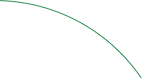
Decreasing Density
PDF starts at λ and decreases exponentially
Mode at 0, right-skewed distribution
Universal Insight: Exponential distribution is the mathematical embodiment of "constant hazard" -
it models situations where the instantaneous rate of occurrence remains constant over time! 🎯
Memoryless Magic: Only continuous distribution where "age doesn't matter"
Parameter Rule: Higher λ means shorter waits, λ = 1/mean_time
Shape Character: Always right-skewed, starts high and decreases rapidly
Practical Test: If mean ≈ standard deviation, consider exponential model